Category Archives: algorithms

Why Data Structures Matter

Our experience on Day 0 of JPR11 yielded a nice example of the need to choose an appropriate implementation of an abstract concept. As I mentioned in the previous post, we experimented with Michael Barker’s Scala implementation of Guy Steele’s parallelizable word-splitting algorithm (slides 51-67). Here’s the core of the issue.

Given a type-compatible associative operator and sequence of values, we can fold the operator over the sequence to obtain a single accumulated value. For example, because addition of integers is associative, addition can be folded over the sequence:

1, 2, 3, 4, 5, 6, 7, 8

from the left:

((((((1 + 2) + 3) + 4) + 5) + 6) + 7) + 8

or the right:

1 + (2 + (3 + (4 + (5 + (6 + (7 + 8))))))

or from the middle outward, by recursive/parallel splitting:

((1 + 2) + (3 + 4)) + ((5 + 6) + (7 + 8))

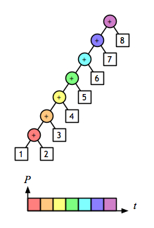
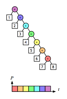
A 2-D view shows even more clearly the opportunity to evaluate sub-expressions in parallel. Assuming that addition is a constant-time operation, the left fold:

foldLeftPlain.jpg

and the right fold:

foldRightPlain.jpg

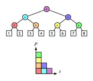
require linear time, but the balanced tree:

foldTreePlain.jpg

can be done in logarithmic time.

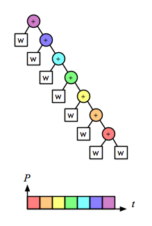
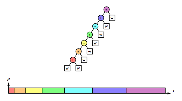
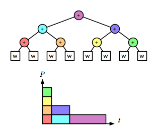
But the associative operation for the word-splitting task involves accumulating lists of words. With a naive implementation of linked lists, appending is not a constant-time operation; it is linear on the length of the left operand. So for this operation the right fold is linear on the size of the task:

foldRightLinear.jpg

the left fold is quadratic:

foldLeftLinear.jpg

and the recursive/parallel version is linear:

foldTreeLinear.jpg

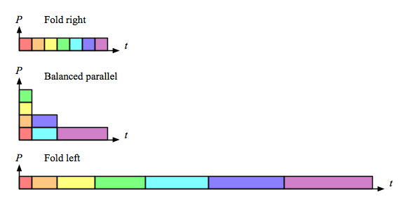
Comparing just the “parallel-activity-versus-time” parts of those diagrams makes it clear that right fold is as fast as the parallel version, and also does less total work:

compareLinear.jpg

Of course, there are other ways to implement the sequence-of-words concept, and that is the whole point. This little example provides a nice illustration of how parallel execution of the wrong implementation is not a win.


The title of this post is a not-very-subtle (but respectful) reference to “Why Functional Programming Matters“, an excellent summary by John Hughes that deserves to be more widely read.

Purely Functional Data Structures, by Chris Okasaki, covers a nice collection of algorithms that avoid the trap mentioned above.

41XlPaC+ZqL._SL160_.jpg

Also, video from this year’s Northeast Scala Symposium is now on-line for the session on functional data structures in Scala, presented by Daniel Spiewak.

Design by proof

The idea of proving programs correct has been around (and hotly debated) for roughly forty years. The irony is that some proof advocates anticipated by more than thirty years what the agile advocates are now saying:

Designing with verification in mind improves the quality of the resulting design.

To be even more specific, compare these statements:

Design the proof,
then write the code so that
it meets the obligations of the proof.
  Write the test first,
then write the code so that
it passes the test.
Edsger Dijkstra   (paraphrased)   Kent Beck   (paraphrased)

I’ve experienced the benefits of following both pieces of advice. Let me apply this approach to a little bit of design which I’ll then use in the Project Euler series. There’s a small amount of algebra involved, but if you don’t want to bother with that, let me request that you at least look at the last section for the punchline.

Sum thing

Consider the following sums, where i in each case ranges from 1 to n:

Power Sum Expanded form Closed form Factored form
0 ∑ i0 1 + 1 + 1 + … + 1 n1 n
1 ∑ i1 1 + 2 + 3 + … + n 1/2 n2 + 1/2 n1 n(n+1)/2
2 ∑ i2 12 + 22 + 32 + … + n2 ?
3 ∑ i3 13 + 23 + 33 + … + n3 ?

Let’s assume that we need the solutions for the last two rows (and Google is down at the moment 😉 ). Using the “designing with verification in mind” approach, we can work them out for ourselves.

Sum of squares

Noticing that ∑ i0 is a polynomial of degree 1, and ∑ i1 is a polynomial of degree 2, we might suspect that the sum of i2 is a polynomial of degree 3. If so, the problem amounts to finding the coefficients for ∑ i2 = an3 + bn2 + cn + d. Let’s assume that as the structure of the solution, and apply test cases to that assumption.

Test case 0: The sum must be zero when n is zero; a03 + b02 + c0 + d = d, therefore d must be zero. That streamlines the polynomial to ∑ i2 = an3 + bn2 + cn.

Test case 1: Adding (n+1)2 to the sum for n must be equal to the result of substituting (n+1) for n in the polynomial.

  an3 + bn2 + cn + (n+1)2
an3 + (b+1)n2 + (c+2)n + 1
and  
  a(n+1)3 + b(n+1)2 + c(n+1)  
an3 + (3a+b)n2 + (3a+2b+c)n +(a+b+c)

These two reduced expressions can only be equal if we can satisfy the equations implied by the coefficients for n2, n1, and n0:

n?   Coefficients   Satisfied if
n2   b+1 = 3a+b   a = 1/3
n1   c+2 = 3a+2b+c   b = 1/2
n0   1 = a+b+c   c = 1/6

So we have a solution of 1/3 n3 + 1/2 n2 + 1/6 n, which we can factor to n(n+1)(2n+1)/6.

Sum of cubes

Based on that success, we’ll pursue the coefficients for ∑ i3 = an4 + bn3 + cn2 + dn + e.

Test case 0: The sum must be zero when n is zero; a04 + b03 + c02 + d0 + e = e, therefore e must be zero, therefore ∑ i3 = an4 + bn3 + cn2 + dn.

Test case 1: Adding (n+1)2 to the sum for n must be equal to the result of substituting (n+1) for n in the polynomial.

  an4 + bn3 + cn2 + dn

+ (n+1)3
an4 + (b+1)n3 + (c+3)n2 + (d+3)n + 1
and  
  a(n+1)4 + b(n+1)3 + c(n+1)2 + d(n+1)  
an4 + (4a+b)n3 + (6a+3b+c)n2 + (4a+3b+2c+d)n + (a+b+c+d)

Again, we look at the coefficients for descending powers of n:

n?   Coefficients   Satisfied if
n3   b+1 = 4a+b   a = 1/4
n2   c+3 = 6a+3b+c   b = 1/2
n1   d+3 = 4a+3b+2c+d   c = 1/4
n0   1 = a+b+c+d   d = 0

So we have a solution of 1/4 n4 + 1/2 n3 + 1/4 n2, which we can factor to (n(n+1)/2)2.

The punchline

“That’s no exponential, that’s my polynomial!” But seriously, folks…

The mathematicians among us–those who haven’t died of boredom–will recognize what we’ve done as an informal (hand-waving) inductive proof.

But I hope that the programmers among us will recognize what we’ve done as test-driven development and (re)factoring. Allowing verification to drive design offers a number of benefits, including:

  • The result itself is verifiable.
  • Each step along the way is more obvious and involves less risk.
  • The result is usually cleaner and more understandable.

Incidentally, I first encountered the term “factoring” applied to programs in Leo Brodie‘s book Thinking Forth (1984). Given my background in Mathematics, it immediately clicked with me. Brodie introduced the idea with a quotation which seems entirely contemporary, once we get past the dated terminology:

“If a module seems almost, but not quite, useful from a second place in the system, try to identify and isolate the useful subfunction. The remainder of the module might be incorporated in its original caller.”

(The quotation is from “Structured Design“, by W.P. Stevens, G.J. Myers, and L.L. Constantine, IBM Systems Journal, vol. 13, no. 2, 1974, © 1974 by International Business Machines Corporation)

As a working developer, I’m excited by the potential of these techniques and the underlying ideas. But as a card-carrying member of the Sid Dabster fan club, I’m constantly amazed at the number of ideas that were actively in play in our field thirty or forty years ago that are now regarded as new, innovative, or even radical.


Recommended reading:

Go with the flow

The second problem from Project Euler asks for the sum of the even Fibonacci numbers which are at most 4,000,000.

An aside on the numbers

The problem’s description of the Fibonacci sequence is flawed (or at least non-standard); the problem statement begins the sequence with 1 and 2, showing the first 10 terms as:

1, 2, 3, 5, 8, 13, 21, 34, 55, 89

It is common to see the definition given as:

fib1 = 1, fib2 = 1, fibn = fibn-1 + fibn-2

I’m persuaded by Dijkstra’s line of reasoning, and prefer to use the definition…

fib0 = 0, fib1 = 1, fibn = fibn-1 + fibn-2

…not only for the benefit of a zero origin, but also because it invites the mind to consider completing the story. The equations…

fibn = fibn-1 + fibn-2

…and…

fibn – fibn-1 = fibn-2

…are clearly equivalent, but the second one may help us realize that we can extend the conventional list to be infinite in both directions…

n -7 -6 -5 -4 -3 -2 -1 0  1  2  3  4  5  6 7
fibn 13 -8 5 -3 2 -1 1 0 1 1 2 3 5 8 13

…making fib a total function over the integers. I’ll put off discussing that interesting option until another time, and for the rest of this post use only natural numbers.

Basic solutions

The naive recursive function for the nth Fibonacci number…

  def fibR(n: Int): Int = {
    if (n == 0)
      0
    else if (n == 1)
      1
    else
      fibR(n - 1) + fibR(n - 2)
  }

…requires O(exp n) time to evaluate. We could go for a tail-recursive (iterative) version…

  def fibI(n: Int): Int = {
    def fib0(i: Int, a: Int, b: Int): Int =
      if (i == n) a else fib0(i + 1, b, a + b)
    fib0(0, 0, 1)
  }

…which executes in O(n) time. That’s an improvement, but still leaves us dealing with the Fibonacci sequence one number at a time.

Gently down the stream

The problem calls for a sum across multiple values from the Fibonacci sequence, and both of the above functions calculate “upwards” to reach the specified value. There’s no point in going through the sequence more than once (regardless of how efficiently we can do that), so let’s think of the sequence as a Stream[Int].

Element-wise addition of streams can be done as:

  def add(s1: Stream[Int], s2: Stream[Int]): Stream[Int] =
       Stream.cons(s1.head + s2.head, plus(s1.tail, s2.tail))

A stream of the Fibonacci numbers is then:

  val fibS: Stream[Int] = Stream.cons(0, Stream.cons(1, add(fibS, fibS tail)))

And now we’re back to familiar territory from the first problem. We simply filter for the even values, apply the limit, and sum the results:

  scala> fibS.filter(_ % 2 == 0).takeWhile(_ <= 4000000).foldLeft(0)(_ + _)
  res17: Int = 4613732

We could stop with that solution, but there are a couple of additional techniques worth a mention.

“Go back, Jack, and do it again”

First, we could replace the stream with a simple Iterator[Int] that holds a pair of consecutive Fibonacci numbers:

  class Fibs extends Iterator[Int] {
    var state = (0, 1)
    def hasNext = true
    def next = {
      val (a, b) = state
      state = (b, a + b)
      a
    }
  }

Thanks to the Iterator trait, when we implement hasNext (is there another value?) and next (return the next value), we get everything needed to complete the solution:

  scala> new Fibs().filter(_ % 2 == 0).takeWhile(_ <= 4000000).foldLeft(0)(_ + _)
  res20: Int = 4613732

However, this still generates three times as many values as needed, because only every third Fibonacci number is even:

0, 1, 1, 2, 3, 5, 8, 13, 21, 34, 55, 89, 144

How could we generate only the even Fibonacci numbers? Notice this progression in the numbers above:

fib0 = 0
fib3 = 2
fib6 = 8
fib9 = 34
fib12 = 144

So we’re interested in producing the sequence fib3n rather than fibn if we want to obtain the even values. In our Fib class above, a and b are consecutive values, fibn and fibn+1. From the original definition, we can apply just a little algebra:

fibn+2 = b + a
fibn+3 = fibn+2 + fibn+1 = (b + a) + b = 2 × b + a
fibn+4 = fibn+3 + fibn+2 = (2 × b + a) + (b + a) = 3 × b + 2 × a

If n is a multiple of 3, then (n + 3) is the next multiple of 3. So the above formulas for fibn+3 and fibn+4 give us a way to write an iterator that produces only even Fibonacci numbers:

  class EvenFibs extends Iterator[Int] {
    var state = (0, 1)
    def hasNext = true
    def next = {
      val (a, b) = state
      state = (2 * b + a, 3 * b + 2 * a)
      a
    }
  }

This new iterator eliminates the need for the filter, reducing the solution to:

  scala> new EvenFibs().takeWhile(_ <= 4000000).foldLeft(0)(_ + _)              
  res30: Int = 4613732

This calculates exactly the values of interest, then uses standard methods to provide the sum. These last three versions retain the ability to re-use the parts that generate the Fibonacci numbers (or even Fibonacci numbers) for purposes other than the sum.

For sake of completeness, here’s the completely optimized version…

  def sumEvenFibs(n: Int) = {
    def iter(a: Int, b: Int, s: Int): Int =
      if (a > n) s else iter(2 * b + a, 3 * b + 2 * a, a + s)
    iter(0, 1, 0)
  }

…which buys performance by giving up that reusability.

Sorting by Schwartzian transform in Scala

The term “Schwartzian transform” was named in honor of Randall Schwartz by Tom Christiansen. (If you recognize either name, you might be thinking, “What would Perl have to do with Scala?” I’ll simply observe that the idea of a multi-paradigm language is an old one.)

At JPR 2008, Dianne Marsh mentioned an article that included a description of the orderby keyword in LINQ. The resulting conversation explored the strategy described below.

The example

Let’s use a minimal Employee class for our discussion:

  class Employee(
      val id:    Int,
      val dept:  String,
      val first: String,
      val last:  String
  ) {
    override def toString() =
      "(" + id + ") " + first + " " + last + " in " + dept
  }

Here’s a list of sample data, used as the basis for a list of employees:

  val data = List(
      (314, "Payroll", "Ursula", "Ficus"),
      (159, "Sales", "Ville", "Eave"),
      (265, "Development", "Wilbur", "Dim"),
      (358, "Sales", "Xeris", "Confabulation"),
      (979, "Development", "Yolanda", "Borg"),
      (323, "Development", "Ziggy", "Ableton")
  )
  val employees =
    for ((id, dp, fn, ln) <- data) yield new Employee(id, dp, fn, ln)

Note that we could mix in the Ordered trait, implementing compare and equals methods, to create a standard ordering for Employee. We won’t use that approach here because we intend to sort employee lists in a variety of ways: alphabetically by name, by employee ID, or even by length of name.

The goal

Our immediate objective is to create a function to sort a list of objects by identifying the sort criteria. The result of the discussion is the sortBy function, which allows us to sort our employees by first name and employee ID by writing as little as:

  sortBy ((e: Employee) => (e.first, e.id)) (employees)

The remainder of this post describes how we compose such a function. There’s certainly room for further enhancement, but getting this far was enough for one conversation (and more than enough for one article).

The standard sort method

Scala’s List class has a pre-defined sort method which uses a caller-provided function to determine whether a pair of elements is in order. To obtain a list sorted by a single Employee attribute, such as id, we can write the expression:

  employees.sort((a, b) => a.id < b.id)

Because it takes only a single argument, the sort method can be written as…

  employees sort ((a, b) => a.id < b.id)

…which is the style I’ll use for the remainder of this article.

Scala also doesn’t require us to specify the type for arguments a and b; the compiler can infer that they have type Employee because they are coming from employees, which has type List[Employee]. (In this case, we could go further and use placeholder syntax to abbreviate the above to…

  employees sort (_.id < _.id)

…but we can’t use that abbreviation for functions that refer to the same parameter more than once.)

As our sorting criteria are more complex (i.e. sorting by length of name, with last name and then first name as tie-breakers), the in-line syntax becomes cumbersome. We can define and use a method which returns Boolean, as in:

  def lessByNameLength(a: Employee, b: Employee): Boolean = {
    val bylength = (a.first + a.last).length - (b.first + b.last).length
    if (bylength == 0) {
      val bylastname = a.last compare b.last
      if (bylastname == 0) {
        a.first < b.first
      } else {
        bylastname < 0
      }
    } else {
      bylength < 0
    }
  }
  // ...
  val employeesByNameLength = employees sort lessByNameLength

That approach provides the per-call flexibility we want, but it has two drawbacks:

  1. it is “boilerplate-heavy”, and
  2. it re-derives the ordering data for each operand, regardless of how many times the operand has been examined previously.

With respect to point #1, the multiple-key comparison requires much more typing, hides our intention in a mound of implementation detail, and is therefore much more error-prone. (For example, if a.first < b.first had been mistyped as a.first > b.first, how long would it take to find the typo-bug?)

We’ll address the boilerplate issue after we discuss the other drawback.

Schwartzian transform

A typical, well-chosen sorting algorithm requires O(n log n) comparisons. The key idea (pun intended) of the Schwartzian transform is to:

  • compute the sort key for each value in the collection and attach it to that value,
  • sort the key/value combinations based on the pre-computed keys, and
  • extract the sorted values from the key/value combinations.

This is a nice application of the time-honored mathematical strategy of transforming a problem to a representation which makes work easier, doing the work, and then transforming the result back (f = g · h · g-1). Each stage can be written and examined individually, a core idea in functional programming. Re #2 above, this approach performs the key computation exactly once per original element, during the setup stage, rather than repeating it every time a pair of elements is compared.

So what do we do with the keys, and how do we use them in the sorting process?

Tuples as keys

A nice feature of Scala tuples is the implicit conversion to Ordered for a tuple whose fields have Ordered types. For example…

  val data = List(
    ("my", 9),
    ("ukulele", 8),
    ("has", 7),
    ("my", 6),
    ("dog", 5),
    ("has", 4),
    ("fleas", 3)
  )
  println(data sort (_ < _))

…produces output of…

  List((dog,5), (fleas,3), (has,4), (has,7), (my,6), (my,9), (ukulele,8))

…in which the values are ordered by the first element of each tuple, with the second element serving to break ties. Because String and Int are both Ordered, Scala can treat Tuple2[String,Int] as Ordered as well.

It’s easy to write a function that produces a key tuple from an instance of Employee, especially if the key is simply made up of fields! Examples of this include:

  def byName       (e: Employee) = (e.last, e.first)
  def byDeptId     (e: Employee) = (e.dept, e.id)
  def byNameLength (e: Employee) = ((e.first + e.last).length, e.last, e.first)

That idea, along with map, zip, and the sort method described earlier, provide all the raw materials we need.

Bolting it together

After reviewing the map and zip methods, we’re ready to start assembling a solution.

If Visitor is the standard illustration for OO design patterns, then map probably fills that role for functional programming. It’s the first syllable in “mapReduce“, and also makes an occasional guest appearance when closures are being discussed.

The expression

  employees map byDeptId 

applies byDeptId to each element of employees and returns the results as a List (which I’ve wrapped to fit on the page):

  List((Payroll,314), (Sales,159), (Development,265),
       (Sales,358), (Development,979), (Development,323))

Associating each key with the corresponding employee is the job of zip, which combines two sequences (as if matching the two sides of a zipper). Given two lists, aList and bList, the expression aList zip bList returns a list of pairs (instances of Tuple2), each of which contains an element of aList and the corresponding element of bList. In our case, that means that…

  employees map byDeptId zip employee

…gives us the list of key/value pairs we need to sort our employees by department and then by ID. Because we want to sort only by the key part of each pair, we need to use sort with a function that compares just the keys. The _1 method retrieves the first element of a Tuple2 instance, so we’ll write:

  employees map byDeptId zip employees sort (_._1 < _._1)

With key/value pairs in the desired order, we are ready to extract the values to form the result, which we can do by adding another map to the pipeline:

  employees map byDeptId zip employees sort (_._1 < _._1) map (_._2)

Evaluating that expression gives us a sorted list. Printed one element per line (via the toString method) it contains:

  (265) Wilbur Dim in Development
  (323) Ziggy Ableton in Development
  (979) Yolanda Borg in Development
  (314) Ursula Ficus in Payroll
  (159) Ville Eave in Sales
  (358) Xeris Confabulation in Sales

Getting functional

Now that we can write an expression that does what we want in a specific instance, we want a general function that captures the core pattern. Looking at the last expression above, it’s clear that the key-extraction function and the list of values are the two parts that need to vary as we re-use the idea. The general template is…

  employees map ? zip ? sort (_._1 < _._1) map (_._2)

…so we just need to fill in the blanks in the following function definition:

  def sortBy ? (f: ?) (vs: ?): ? = {
    (vs map f zip vs) sort (_._1 < _._1) map (_._2)
  }

If the values (the vs parameter) are provided in a list of some type, then the result should be a list of the same type. Because that type can very, we will use type parameters. Choosing V for our value type, we get:

  def sortBy[V, ?] (f: V => ?) (vs: List[V]): List[V] = {
    (vs map f zip vs) sort (_._1 < _._1) map (_._2)
  }

Specifying the remaining type parameter is a bit tricky; we need for f to map from type V to type K (for key)…

  def sortBy[V, K ?] (f: V => K) (vs: List[V]): List[V] = {
    (vs map f zip vs) sort (_._1 < _._1) map (_._2)
  }

…however, K must be a type we can sort. As mentioned in the “Tuples as keys” section, Scala has an implicit conversion to Ordered for tuples (for Tuple2 through Tuple9, actually). That means that we must specify that K can be converted implicitly to Ordered[K], which give us the last bit of type incantation:

  def sortBy[V, K <% Ordered[K]] (f: V => K) (vs: List[V]): List[V] = {
    (vs map f zip vs) sort (_._1 < _._1) map (_._2)
  }

While that last detail is not the sort of thing you’d likely want to write throughout your application code, you don’t have to! That last definition is the sort of thing (pun intended 😉 that you’d put in a library (utility jar, etc.) and just use throughout your application. With that function in hand, we’re now free to write…

  val sortedEmps = sortBy ((e: Employee) => (e.first, e.id)) (employees)

…or…

  def byNameLength (e: Employee) = ((e.first + e.last).length, e.last, e.first)
  // ...
  val sortedEmps = sortBy (byNameLength)(employees)

…or even…

  def byNameLength (e: Employee) = ((e.first + e.last).length, e.last, e.first)
  def sortEmployeesByNameLength = sortBy (byNameLength) _
  // ...
  val sortedEmps = sortEmployeesByNameLength(employees)

…if you’ve read the post on currying, that is.